Alexander Fabisch - Learning Curves in scikit learn

scikit learn is a great machine learning library for Python. It offers broad range of machine learning algorithms and tools. Learning curves are a new tool that has been merged last week and I want to use that feature to point out why scikit learn is such a great library.

A learning curve shows the training scores and the test scores for varying number of training samples. It is a tool that can be used to find out whether we benefit from more training samples. At a first look, it seems to be very easy to implement. We could do something like:

estimator = ...
X_train, y_train, X_test, y_test = split(X, y)
n_samples = X_train.shape[0]
train_scores, test_scores = [], []
for n in range(10, 10, n_samples):
    estimator.fit(X_train[:n], y_train[n])
    train_scores.append(estimator.score(X_train[:n], y_train[n]))
    test_scores.append(estimator.score(X_test, y_test))
plot(range(10, 10, n_samples), train_scores)
plot(range(10, 10, n_samples), test_scores)

However, there are some flaws in the code that make the implementation actually much worse than the version that is implemented in scikit learn:

We have to define the split function.
Actually, real cross-validation would be even better to generate more stable learning curves. But that would require an additional loop and afterwards averaging over the runs. (Fortunately, scikit learn could generate the cross-validation splits for us: sklearn.cross_validation.)
If we would like to use another scoring, we would have to change that in the code. Fortunately, scikit-learn comes already with a wide range of predefined scorers in sklearn.metrics.
We can parallelize over cross-validation runs and different numbers of training samples and that would require even more code.
Incremental learning could be exploited! If we would like to train an online learning algorithm like sklearn.linear_model.SGDClassifier on a large dataset, we can reuse models that have been fitted on parts of the training set to speed up the generation of the learning curve.
This works only for supervised learning. We can of course compute scores for unsupervised learners like clustering algorithms but that would require additional code.
Maybe we are not interested in the exact number of training examples but want something like a plot for 10%, 20%, ..., 100% of the training examples.

The three required arrays that are used to actually plot the curves can be generated in just one call to sklearn.learning_curve.learning_curve without all these flaws.

Lets take a look at the signature of the function learning_curve:

train_sizes_abs, train_scores, test_scores = \
    learning_curve(estimator, X, y,
                   train_sizes=np.linspace(0.1, 1.0, 10),
                   cv=None, scoring=None,
                   exploit_incremental_learning=False,
                   n_jobs=1, pre_dispatch="all", verbose=0)

It takes an estimator and the whole training set (X, y) where y could be None. We already have a good default for train_sizes: an array with dtype == float is interpreted as fractions of the maximum number of training examples, i.e. the default is like 10%, 20%, ..., 100%. Otherwise the sizes are interpreted as absolute numbers of training samples. We can set some standard parallelization options for joblib like n_jobs and pre_dispatch and we can even exploit incremental learning.

But the magic happens in the arguments cv and scoring. These parameters rely on the huge feature range of scikit learn. cv can be a cross-validation generator like sklearn.cross_validation.KFold, a list of train and test indices for each test run or just an integer that is interpreted as the number of folds for k-fold cross-validation. If the estimator is a classifier it will be interpreted as the number of folds for stratified k-fold cross-validation. scikit learn supports even more cross-validation methods like leave-one-out CV etc. The default value (None) will be interpreted as 3-fold cross-validation.

Similar things happen with the scoring parameter. If it is None, the function assumes that there is a member function estimator.score. We can also pass a callable with the signature scorer(estimator, X[, y]) or a string that will be mapped to a built-in scorer like for example r2, accuracy or precision_scorer. Note that the scorer could also compute scores for unsupervised learners.

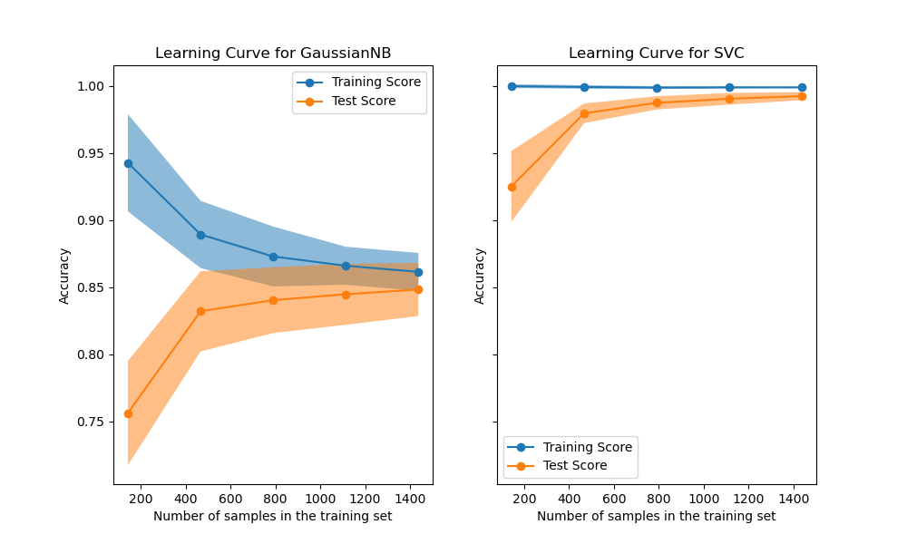
With only a few lines of code we can now plot beautiful learning curves like these:

scikit learn offers many more tools like this, for example model selection with grid search or random search, a pipeline that combines preprocessing and learners, simple dataset access and dataset generators and a really great explanatory documentation.