Artificial Neural Networks
%pylab inline
from mpl_toolkits.mplot3d import Axes3D
What is Backprop?
- We have to optimize \(\boldsymbol{w}\) such that \(E\) is at a minimum.
- Backprop is a procedure to compute the gradient of the error function with respect to the weights of a neural network.
- We can use the gradient from backprop to apply gradient descent.

Learning ANNs
from IPython.display import YouTubeVideo
YouTubeVideo("MkLJ-9MubKQ")
print YouTubeVideo("MkLJ-9MubKQ").src
Difficulties
- There are many local minima.
- The optimization problem is ill-conditioned.
- There are many flat regions (saddle points).
- There is no guarantee to reach the global minimum.
- Deep architectures suffer from the vanishing gradient problem.
- Neural networks are usually considered to be the blackest box of all learning algorithms.
- There are sooo many hyperparameters (number of layers/nodes, activation function, connectivity, weight initialization, loss function, regularization, ...).
- Training neural networks has been regarded as black magic by many researchers.
- And here is the grimoire: Neural Networks: Tricks of the Trade (1st edition: 1998; 2nd edition: 2012).
However, there have been three hypes around ANNs:
- Perceptron (50s-XOR problem)
- Backpropagation (80s-SVM)
- Deep Learning (2006-now)
And they work incredibly well in practice.
XOR Problem
# Dataset
X = array([[0, 1], [1, 0], [0, 0], [1, 1]])
Y = array([1, 1, 0, 0])
N = Y.shape[0]

scatter(X[:, 0], X[:, 1], c=Y, cmap=cm.gray, s=100)
r = setp(gca(), xticks=(), yticks=())

Error Surface of the XOR Problem
Activation function
def logit(a): return 1.0/(1+exp(-a))
Forward propagation for 2 inputs (x1, x2), 2 hidden nodes, 1 output
def fprop(x1,x2,w1=0.1,w2=0.2,b1=0.1,w3=-0.2,w4=0.2,b2=-0.1,w5=-0.3,w6=-0.25,b3=0.2):
    return logit(b1+w1*logit(b2+w3*x1+w4*x2)+w2*logit(b3+w5*x1+w6*x2))
i, j = 4, 5 # Weight indices
fig = figure(figsize=(8, 6))
W1, W2 = meshgrid(arange(-10, 10, 0.25), arange(-10, 10, 0.25))
E = numpy.sum([(fprop(X[n, 0], X[n, 1], **{"w%d"%(i+1) : W1, "w%d"%(j+1) : W2})-Y[n])**2
               for n in range(N)], axis=0)
ax = fig.add_subplot(111, projection="3d")
surf = ax.plot_surface(W1, W2, E, rstride=1, cstride=1,
                       cmap=cm.coolwarm, lw=0)
setp(ax, xticks=(), yticks=(), zticks=(),
     xlabel="$w_%d$" % (i+1), ylabel="$w_%d$" % (j+1), zlabel="E")
matplotlib.rcParams.update({"font.size": 20})

Application of the Week: Handwritten Digit Recognition
- THE MNIST DATABASE of handwritten digits
- 28x28 = 784 pixels
- 60,000 examples for training
- 10,000 examples for testing
- (MNIST can be considered as "solved" and is now a standard benchmark.)
import sys
sys.path.append("03_ann")
from mnist import read
images, labels = read(range(10), 'testing', path="03_ann")
nrows, ncols = (15, 24)
figure(figsize=(ncols/3, nrows/3))
subplots_adjust(left=0.0, bottom=0.0, right=1.0, top=1.0, wspace=0.0, hspace=0.0)
for i in range(nrows*ncols):
    setp(subplot(nrows, ncols, i+1), xticks=[], yticks=[])
    imshow(images[i], cmap=cm.gray, interpolation="nearest")

Convolutional Neural Network (CNN)

Convolution
import pickle
from tools import scale, model_accuracy

X_mnist = scale(images)[:, newaxis, :, :]
net = pickle.load(open("03_ann/cnn.pickle", "rb"))
print "Accuracy on MNIST test set: %.2f %%" % (100*model_accuracy(net, X_mnist, labels))
nrows, ncols = 3, 5
matplotlib.rcParams.update({"font.size": 10})
figure(figsize=(1.5*ncols, 1.5*nrows))
subplots_adjust(left=0.0, bottom=0.0, right=1.0, top=1.0, wspace=0.05, hspace=0.15)
i = j = 0
while j < ncols*nrows:
    p, a = net.predict([X_mnist[i]]).ravel().argsort()[::-1], labels[i]
    if p[0] != a:
        setp(subplot(nrows, ncols, j+1), xticks=[], yticks=[])
        title("P. %d, %d, %d / A. %d" % (p[0], p[1], p[2], a))
        imshow(images[i], cmap=cm.gray, interpolation="nearest")
        j += 1
    i += 1

Artificial Neuron

Neuron
Multilayer Neural Network
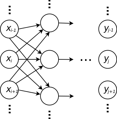
Layers
The Original Fprop/Backprop Formulas
Fprop
In each layer
\[a_j = \sum_i w_{ji} x_i\] \[y_j = g(a_j)\]
where
- \(y_j\) is the \(j\)th output
- \(x_i\) is the \(i\)th input
- \(w_{ji}\) is the weight
- \(a_{j}\) is called activation
- \(g\) is the activation function, e.g. \(\tanh\) in the hidden layers and the identity in the last layer (for regression)
Error function (SSE)
\[E = \frac{1}{2} \sum_n \sum_j \left( y_j^{(n)} - t_j^{(n)} \right)^2\]
Backprop
In each layer (we will omit the sample index \(n\))
\[\delta_j = \begin{cases}y_j - t_j & \text{in the output layer}\\\\ g'(a_j) \sum_k \frac{\partial E}{\partial y_k} & \text{otherwise}\end{cases},\]
\[\frac{\partial E}{\partial w_{ji}} = \delta_j x_i\]
\[\frac{\partial E}{\partial x_i} = \delta_j w_{ji}\]
where
- all nodes \(k\) are in the layer after \(j\)
- \(a_j\) is known from fprop: \(\sum_i w_{ji} x_i\)
- actually you do not have to save \(a_j\) because \(g'(a_j)\) usually can be computed from \(y_j\), e.g.
- identity function: \(g'(a_j) = 1\)
- \(\tanh\): \(g'(a_j) = 1 - y_j^2\)
- \(\frac{\partial E^{(n)}}{\partial w_{ji}}\) will be used to update the weight \(w_{ji}\) in gradient descent
- \(\frac{\partial E^{(n)}}{\partial x_i}\) will be passed to the previous layer to compute the deltas
Do not forget to sum up the gradient with respect to the weights for each training example!
Efficient Fprop/Backprop Implementation for Fully Connected Layers
- Make sure that you have an efficient linear algebra library.
- Organize your data in matrices, i.e.
- The matrix \(\boldsymbol{X}\) contains an input vector in each row. Note that you must expand each row by the bias 1.
- The matrix \(\boldsymbol{T}\) contains an output (of the network) in each row.
- Each layer should have the functions
fprop(W, X, g) -> Ybackprop(W, X, g_derivative, Y, dE/dY) -> dE/dX, dEdW
Efficient Fprop
In each layer
\[\boldsymbol{A} = \boldsymbol{X} \boldsymbol{W}^T\] \[\boldsymbol{Y} = g(\boldsymbol{A})\]
where
- \(\boldsymbol{Y} \in \mathbb{R}^{N \times J}\) contains an output vector in each row, i.e. \(\boldsymbol{Y}_{nj} = y^{(n)}_j\)
- \(\boldsymbol{X} \in \mathbb{R}^{N \times I}\) contains an input vector (the output of the previous layer) in each row, i.e. \(\boldsymbol{X}_{ni} = x^{(n)}_i\)
- \(\boldsymbol{W} \in \mathbb{R}^{J \times I}\) is the weight matrix of the layer, i.e. \(\boldsymbol{W}_{ji}\) is the weight between input \(i\) and output \(j\).
- \(g\) is the activation function (implemented to work with matrices)
- \(I\) is the number of inputs, i.e. the number of outputs of the previous layer plus 1 (for the bias)
- \(J\) is the number of outputs
Make sure that you add the bias entry in each row before you pass \(Y\) as input to the next layer!
Error function (SSE)
\[E = \frac{1}{2} ||\boldsymbol{Y} - \boldsymbol{T}||_2^2\]
where
- \(||.||_2\) is the Frobenius norm.
Efficient Backprop
In each layer
\[\Delta = g'(\boldsymbol{A}) * \frac{\partial E}{\partial \boldsymbol{Y}}\] \[\frac{\partial E}{\partial \boldsymbol{W}} = \Delta^T \cdot \boldsymbol{X}\] \[\frac{\partial E}{\partial \boldsymbol{X}} = \Delta \cdot \boldsymbol{W}\]
where
- \(*\) is the Hadamard product or Schur product or entrywise product
- \(\frac{\partial E}{\partial \boldsymbol{Y}}\) contains derivatives of the error function with respect to the outputs (\(\boldsymbol{Y} - \boldsymbol{T} = \frac{\partial E}{\partial \boldsymbol{Y}}\) in the last layer)
- \(\frac{\partial E}{\partial \boldsymbol{X}} \in \mathbb{R}^{N \times I}\) contains derivatives of the error function with respect to the inputs and will be passed to the previous layer
- \(\Delta \in \mathbb{R}^{N \times J}\) contains deltas: \(\delta_j^{(n)} = \Delta_{jn}\)
- \(g'\) is the derivative of \(g\) and can be computed based only on \(\boldsymbol{Y}\)
- \(\frac{\partial E}{\partial \boldsymbol{W}} \in \mathbb{R}^{J \times I}\) contains the derivatives of the error function with respect to \(\boldsymbol{W}\) and will be used to optimize the weights of the ANN
Make sure that you remove the bias entry in each row before you pass \(\frac{\partial E}{\partial \boldsymbol{X}}\) to the previous layer!
Tips for Your Implementations
- Check your gradients.
- Check your gradients.
- Check your gradients.
- With finite differences: \[\frac{\partial E^{(n)}}{\partial w_{ji}} = \frac{E^{(n)}(w_{ji} + \epsilon) - E^{(n)}(w_{ji} - \epsilon)}{2 \epsilon} + \mathcal{O}(\epsilon^2)\]
Question 1
- How should we initialize the weights \(\boldsymbol{w}\)?
Answer 1
- Draw components of \(\boldsymbol{w}\) iid (independend and identically distributed) from a Gaussian distrubition with small standard deviation, e.g. 0.05.
- Initialization with 0 will prevent the gradient from flowing back to the lower layers: \[\frac{\partial E}{\partial x_i} = \delta_j w_{ji}\]
random.randn(10) * 0.05
Derivatives of Activation Functions
- Identity
\[y = g(a) = a\] \[g'(a) = 1\]
- Hyperbolic tangent
\[y = g(a) = \tanh(a)\] \[g'(a) = 1 - \tanh^2(a) = 1-y^2\]
- Logistic function
\[y = g(a) = \frac{1}{1+\exp{-a}}\] \[g'(a) = g(a) (1 - g(a)) = y (1-y)\]
def plot_afun(x, y, sp_idx, label=None):
    """Plot activation function."""
    ax = subplot(2, 4, sp_idx)
    if label is not None: title(label)
    setp(ax, xlim=(min(x), max(x)), ylim=(min(y)-0.5, max(y)+0.5))
    plot(x, y)

figure(figsize=(10, 4))
x = linspace(-5, 5, 100)
plot_afun(x, x, 1, label="Identity")
plot_afun(x, tanh(x), 2, label="tanh")
plot_afun(x, logit(x), 3, label="Logistic Function")
plot_afun(x, numpy.max((x, zeros_like(x)), axis=0), 4, label="Rectified Linear Unit (ReLU)")
plot_afun(x, ones_like(x), 5)
plot_afun(x, 1-tanh(x)**2, 6)
plot_afun(x, logit(x)*(1-logit(x)), 7)
plot_afun(x, numpy.max((sign(x), zeros_like(x)), axis=0), 8)

Why do neural nets work so well in practice?
- We don't want to find the global minimum. Overfitting!
- SGD finds sufficiently good local minima.
- Neural nets learn feature hierarchies to represent functions efficiently.
Escaping Local Minima with SGD
i, j = 4, 5

figure(figsize=(12, 4))
W = arange(-10, 10, 0.25)
errors = [(fprop(X[n, 0], X[n, 1], **{"w%d"%(i+1) : W, "w%d"%(j+1) : W+2})-Y[n])**2
          for n in range(N)]
subplot(1, 2, 1)
for n in range(N): plot(W, errors[n], label="$E_%d$" % n)
setp(gca(), xticks=(), yticks=(), xlabel="$w$", ylabel="E")
legend(loc="best")
subplot(1, 2, 2)
plot(W, numpy.sum(errors, axis=0), label="E")
setp(gca(), xticks=(), yticks=(), xlabel="$w$", ylabel="E")
legend(loc="best")

Question 2
What are advantages and drawbacks in comparison to other regression and classification algorithms?
For example:
- linear regression, logistic regression
- SVR, SVM
- decision trees
- k-nearest neighbors
Answer 2
Drawbacks
- input has to be a vector of real numbers, e.g. text must be converted befor classification
- in general, the optimization problem is very difficult because it is ill-conditioned and non-separable
- objective function is not convex, there are many local minima and flat regions
- black box: in most cases it is very difficult to interpret the weights of a neural network although it is possible!
- catastrophic forgetting: learning one instance can change the whole network
Advantages
- universal function approximator, nonlinear functions can be represented
- can learn smooth functions
- features will be learned automatically
- allows learning of hierarchical features which is much more efficient than just one layer of abstraction
- multiclass classification can be integrated with linear complexity (softmax activation function, cross-entropy error function)
- it is a parametric model, it does not store any training data directly